
[solved]-Use Sampling Distribution Applet Statcrunch Investigate Properties Sampling Distributions Q39022687
The graphs and data attached at the end. Thanks 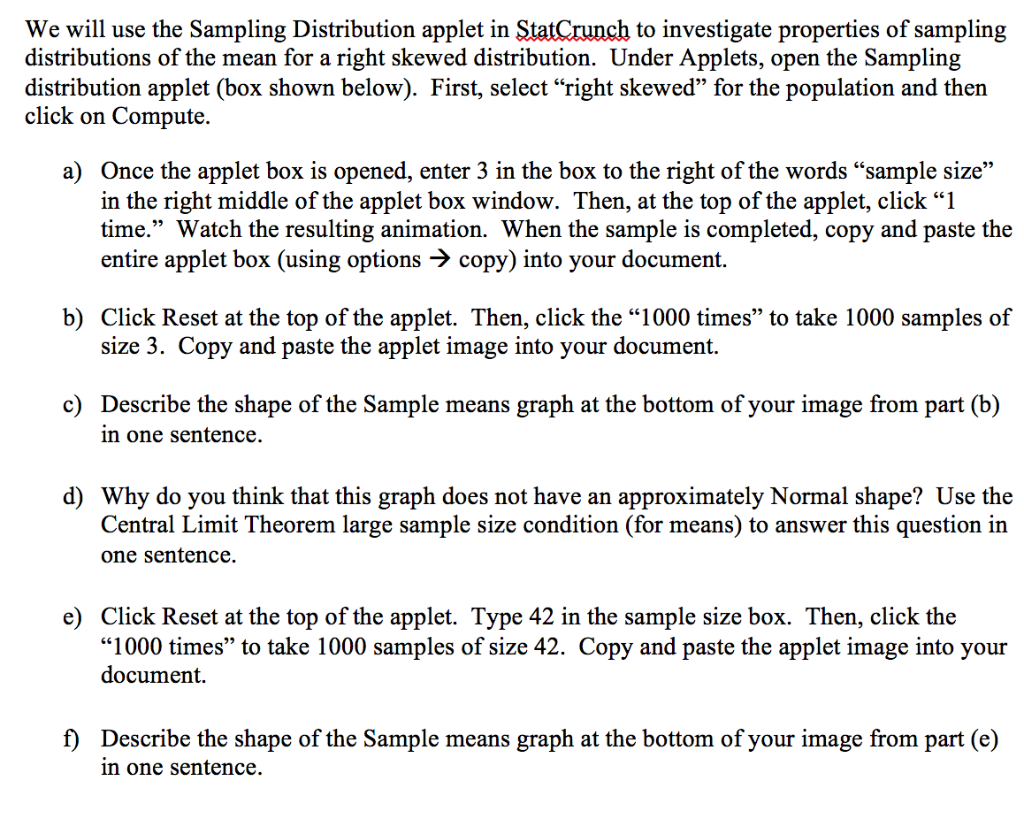

We will use the Sampling Distribution applet in StatCrunch to investigate properties of sampling distributions of the mean for a right skewed distribution. Under Applets, open the Sampling distribution applet (box shown below). First, select “right skewed” for the population and then click on Compute. a) Once the applet box is opened, enter 3 in the box to the right of the words “sample size” in the right middle of the applet box window. Then, at the top of the applet, click “1 time.” Watch the resulting animation. When the sample is completed, copy and paste the entire applet box (using options → copy) into your document. b) Click Reset at the top of the applet. Then, click the “1000 times” to take 1000 samples of size 3. Copy and paste the applet image into your document. c) Describe the shape of the Sample means graph at the bottom of your image from part (b) in one sentence. d) Why do you think that this graph does not have an approximately Normal shape? Use the Central Limit Theorem large sample size condition (for means) to answer this question in one sentence. e) Click Reset at the top of the applet. Type 42 in the sample size box. Then, click the “1000 times” to take 1000 samples of size 42. Copy and paste the applet image into your document. f) Describe the shape of the Sample means graph at the bottom of your image from part (e) in one sentence. g) Why do you think that this graph from part (f) has the shape you described? Use the Central Limit Theorem large sample size condition to answer this question in one sentence. h) Using the image in part (e), write the values you obtained for the mean (in green) and the standard deviation (in blue). These values are found in the bottom right box labeled “Sample Means” i) Compare the mean value in green, found in part (h) to the known mean of the population from the top box labeled “Population.” j) Now calculate the standard error of the sample mean using the value labeled “Std. dev.” in blue from the top box. Round this value to three decimal places. k) Compare the value in part (j) to the standard deviation (in blue) you obtained in part (h) in one sentence. Assuming this right skewed population distribution had a population mean of 14.05 and a standard deviation of 11.83; calculate the probability that, in a random sample of 42, the mean of the sample is greater than 15. First, draw a picture with the mean labeled, shade the area representing the desired probability, standardize, and use the Standard Normal Table (Table 2 in your text) to obtain this probability. Please take a picture of your hand drawn sketch and upload it to your Word document (if you do not have this technology, you may use any other method (i.e. Microsoft paint) to sketch the image). You must type the rest of your “by hand”. || Sampling Distributions Population Mean Median Std. dev. 14.0519 10.7484 11.8255 = 10 20 30 40 50 Population Samples Sample size Mean Median Std. dev. 26.5545 33.694 14.8147 10 20 30 Samples 40 50 Sample means # of Samples Mean 26.5545 Median 26.5545 Std. dev. 10 20 30 40 50 Sample means Sampling Distributions Population Mean Median Std. dev. 14.0519 10.7484 11.8255 Ő 10 20 30 40 50 Population iMHO Samples Sample size Mean Median Std. dev. 17.4531 19.3597 12.3425 10 30 40 50 Samples Sample means # of 1000 Samples Mean 13.9711 Median 13.0295 Std. dev. 6.9904 10 20 30 Sample means 40 50 Sampling Distributions Population Mean Median Std. dev. 14.0519 10.7484 11.8255 0 10 20 30 Population 40 50 Samples Sample size Mean Median Std. dev. 42 13.3659 11.4148 10.0921 10 20 30 Samples 40 50 2007 1507 1000 100+ Sample means # of Samples Mean Median Std. dev. 14.0079 14.0279 1.8236 0 10 20 30 Sample means 40 50 Show transcribed image text We will use the Sampling Distribution applet in StatCrunch to investigate properties of sampling distributions of the mean for a right skewed distribution. Under Applets, open the Sampling distribution applet (box shown below). First, select “right skewed” for the population and then click on Compute. a) Once the applet box is opened, enter 3 in the box to the right of the words “sample size” in the right middle of the applet box window. Then, at the top of the applet, click “1 time.” Watch the resulting animation. When the sample is completed, copy and paste the entire applet box (using options → copy) into your document. b) Click Reset at the top of the applet. Then, click the “1000 times” to take 1000 samples of size 3. Copy and paste the applet image into your document. c) Describe the shape of the Sample means graph at the bottom of your image from part (b) in one sentence. d) Why do you think that this graph does not have an approximately Normal shape? Use the Central Limit Theorem large sample size condition (for means) to answer this question in one sentence. e) Click Reset at the top of the applet. Type 42 in the sample size box. Then, click the “1000 times” to take 1000 samples of size 42. Copy and paste the applet image into your document. f) Describe the shape of the Sample means graph at the bottom of your image from part (e) in one sentence.
g) Why do you think that this graph from part (f) has the shape you described? Use the Central Limit Theorem large sample size condition to answer this question in one sentence. h) Using the image in part (e), write the values you obtained for the mean (in green) and the standard deviation (in blue). These values are found in the bottom right box labeled “Sample Means” i) Compare the mean value in green, found in part (h) to the known mean of the population from the top box labeled “Population.” j) Now calculate the standard error of the sample mean using the value labeled “Std. dev.” in blue from the top box. Round this value to three decimal places. k) Compare the value in part (j) to the standard deviation (in blue) you obtained in part (h) in one sentence. Assuming this right skewed population distribution had a population mean of 14.05 and a standard deviation of 11.83; calculate the probability that, in a random sample of 42, the mean of the sample is greater than 15. First, draw a picture with the mean labeled, shade the area representing the desired probability, standardize, and use the Standard Normal Table (Table 2 in your text) to obtain this probability. Please take a picture of your hand drawn sketch and upload it to your Word document (if you do not have this technology, you may use any other method (i.e. Microsoft paint) to sketch the image). You must type the rest of your “by hand”. ||
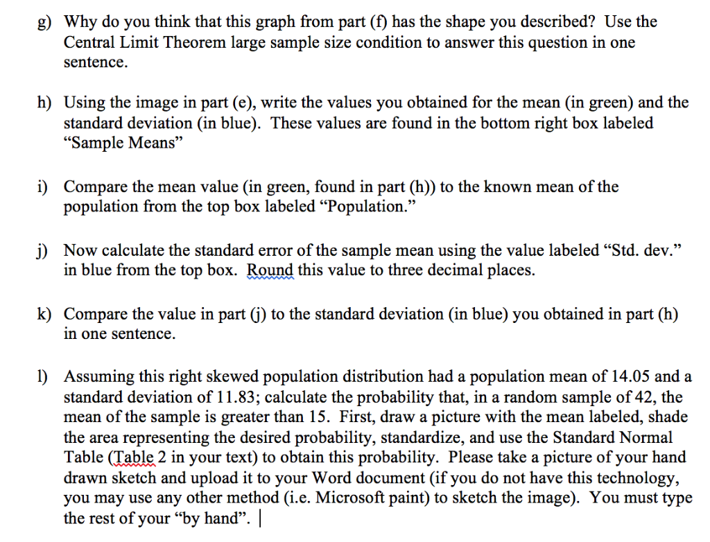
Sampling Distributions Population Mean Median Std. dev. 14.0519 10.7484 11.8255 = 10 20 30 40 50 Population Samples Sample size Mean Median Std. dev. 26.5545 33.694 14.8147 10 20 30 Samples 40 50 Sample means # of Samples Mean 26.5545 Median 26.5545 Std. dev. 10 20 30 40 50 Sample means
Sampling Distributions Population Mean Median Std. dev. 14.0519 10.7484 11.8255 Ő 10 20 30 40 50 Population iMHO Samples Sample size Mean Median Std. dev. 17.4531 19.3597 12.3425 10 30 40 50 Samples Sample means # of 1000 Samples Mean 13.9711 Median 13.0295 Std. dev. 6.9904 10 20 30 Sample means 40 50
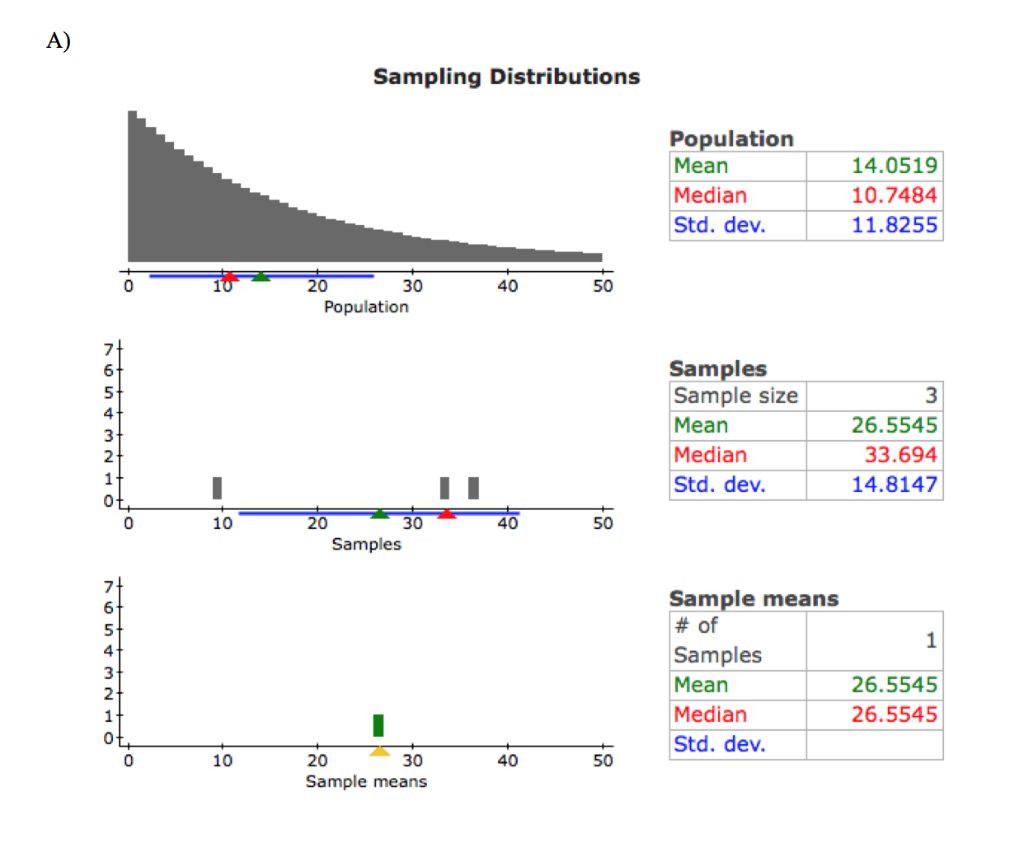
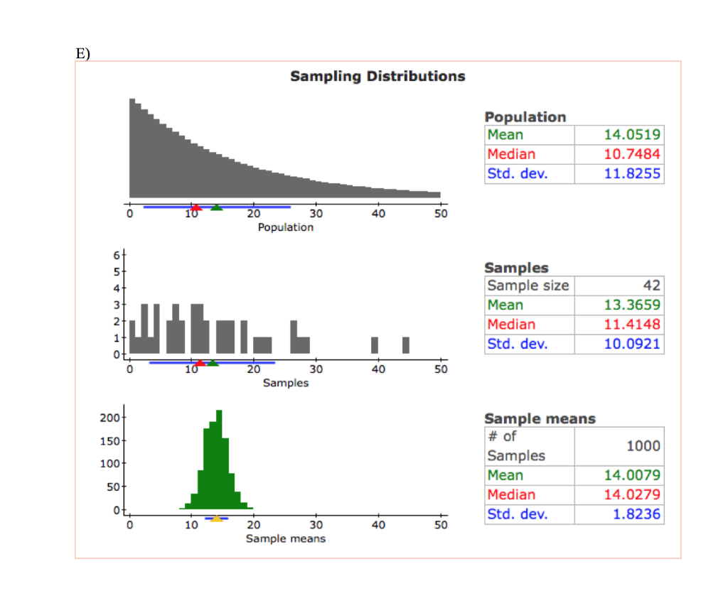
Sampling Distributions Population Mean Median Std. dev. 14.0519 10.7484 11.8255 0 10 20 30 Population 40 50 Samples Sample size Mean Median Std. dev. 42 13.3659 11.4148 10.0921 10 20 30 Samples 40 50 2007 1507 1000 100+ Sample means # of Samples Mean Median Std. dev. 14.0079 14.0279 1.8236 0 10 20 30 Sample means 40 50
Expert Answer
Answer to The graphs and data attached at the end. Thanks … . . .
OR