
[Solved]823 Obtain Parallel Realization Transfer Function Matrix Presented Example 815 Question Ob Q37231214
8.23 Obtain a parallel realization for the transferfunction matrix presented in the above example 8.15
The question is to obtain a parallel realization forthe transfer function matrix presented in the photos
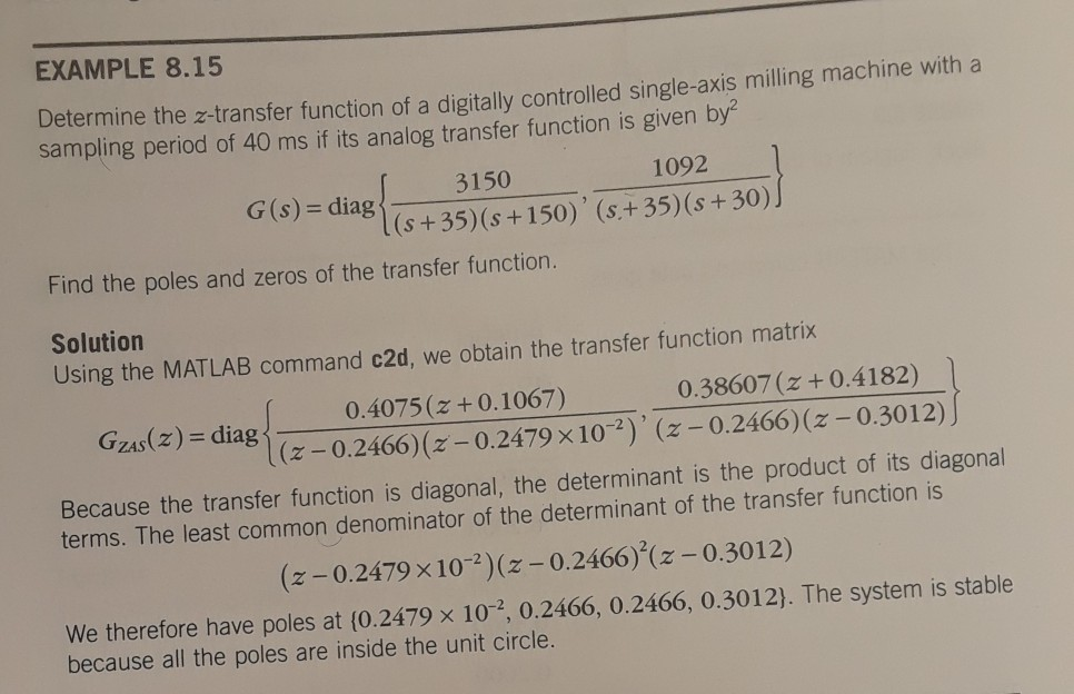
EXAMPLE 8.15 machine with a Determine the z-transfer function of a digitally controlled single-axis milling sampling period of 40 ms if its analog transfer function is given by 1092 3150 G(s) – diag 1 (s + 35)(s +150)’ (s.+ 35) (s +30) Find the poles and zeros of the transfer function. Solution Using the MATLAB command c2d, we obtain the transfer function matrix 0.38607 (z+0.4182) 0.4075 (z + 0.1067) diag(z-0.2466) (z -0.2479 X 10)2-0.2466)(-0.3012) Because the transfer function is diagonal, the determinant is the product of its diagonal terms. The least common denominator of the determinant of the transfer function is (z -0.2479 X 10²)(z -0.2466) (z -0.3012) We therefore have poles at (0.2479 x 10², 0.2466, 0.2466, 0.3012). The system is stable because all the poles are inside the unit circle. To obtain the zeros of the system, we rewrite the transfer function in the form (z- 0.2466) Gadz) = (zー0.2466)2(z-0.2479 × 10⁻²)(z-0.3012) 「04075 (z +0.1067)(z-0.3012) 0 0 0.38607 (z + 0.4182) (z-0.2479 × 10⁻⁹] For this square 2-input-2-output system, the determinant of the transfer function is (Z + 0.1 067) (z-0.301 2)(z +0.4 182)(~_ 0.2479 x 10⁻²)(~_ 0.2466)2 (z – 0.2466) (z 0.2479 x 10²)(z -0.3012)2 (z + 0.1067) (z + 0.4182) (z-0.2466) (z – 0.2479 x10²)(z-0.3012) The roots of the numerator are the zeros (-0.1067, -0.4182) The same answer is obtained using the MATLAB command tzero Show transcribed image text EXAMPLE 8.15 machine with a Determine the z-transfer function of a digitally controlled single-axis milling sampling period of 40 ms if its analog transfer function is given by 1092 3150 G(s) – diag 1 (s + 35)(s +150)’ (s.+ 35) (s +30) Find the poles and zeros of the transfer function. Solution Using the MATLAB command c2d, we obtain the transfer function matrix 0.38607 (z+0.4182) 0.4075 (z + 0.1067) diag(z-0.2466) (z -0.2479 X 10)2-0.2466)(-0.3012) Because the transfer function is diagonal, the determinant is the product of its diagonal terms. The least common denominator of the determinant of the transfer function is (z -0.2479 X 10²)(z -0.2466) (z -0.3012) We therefore have poles at (0.2479 x 10², 0.2466, 0.2466, 0.3012). The system is stable because all the poles are inside the unit circle.
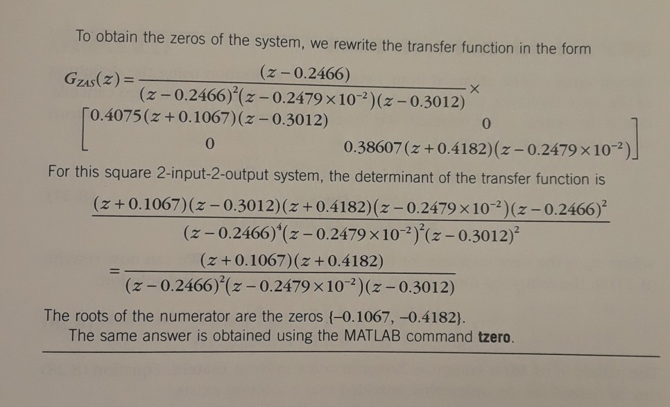
To obtain the zeros of the system, we rewrite the transfer function in the form (z- 0.2466) Gadz) = (zー0.2466)2(z-0.2479 × 10⁻²)(z-0.3012) 「04075 (z +0.1067)(z-0.3012) 0 0 0.38607 (z + 0.4182) (z-0.2479 × 10⁻⁹] For this square 2-input-2-output system, the determinant of the transfer function is (Z + 0.1 067) (z-0.301 2)(z +0.4 182)(~_ 0.2479 x 10⁻²)(~_ 0.2466)2 (z – 0.2466) (z 0.2479 x 10²)(z -0.3012)2 (z + 0.1067) (z + 0.4182) (z-0.2466) (z – 0.2479 x10²)(z-0.3012) The roots of the numerator are the zeros (-0.1067, -0.4182) The same answer is obtained using the MATLAB command tzero
Expert Answer
Answer to 8.23 Obtain a parallel realization for the transfer function matrix presented in the above example 8.15 The question is … . . .
OR